IT News & Technology update

Provide comprehensive update related to Computer, technology, software, anti virus and another electric device

Excel tips: Excel don't calculate automatically

Written by IT News on 10:40 PM

In excel, it’s usually will automatically calculate when applying formulas in selected ranges of cells. If it not, then this simple tips will help you to solve this calculation problem.

  • 1. open Microsoft excel;
    2. Select option from the Tools menu;
    3. Within the option dialog window, navigate to Calculation tab;
    4. If the calculation set to manual now select Automatic;
    5. Click OK,


Note: this tips tested in Microsoft office 2003
If this tips doesn't help this issue please let me know.

Sharing Excel files safely

Written by IT News on 10:20 PM

Sharing an Excel documents is easy. Probably a lot of people don't realize it, but Microsoft built Office 2003 and Office 2007 with collaboration in mind. Both versions allow you to share an Excel workbook with other users so multiple users can make modifications to a spreadsheet. In this article, will show you how to share an Excel 2007 workbook. More importantly, It will discuss how you can keep a shared workbook secure.

Before you start sharing a workbook, the first thing you have to do is protect the spreadsheet you've created. It is very important to lock the cells so that other users are not able to modify them without your permission.

You can protect a range of cells by selecting them, right clicking on them and selecting the Format Cells command from the resulting shortcut menu. When you do, Windows will display the Custom Lists properties sheet. Go to the Protection tab and either lock or unlock the protected cells. Keep in mind that locking a cell has no effect until you protect the sheet.

To protect a worksheet, click on the Review menu and then click the Protect Sheet icon. When you do, Windows will display the Protect Sheet dialog box.

Verify that the Protect Worksheet and Contents of Locked Cells check box is selected. Then enter a password to use in order to unprotect the sheet. Keep in mind that this password is worksheet specific.

Before you click OK, read through the other protection options on this dialog box. You can control what users will and will not be allowed to do to the spreadsheet just by selecting a check box. By default, users are allowed to select both locked and unlocked cells in a protected spreadsheet, but that's about it. It is up to you to decide whether you want to allow your users to format or create or delete cells, rows or columns. You can also authorize or forbid various other types of edits.

Now that you have implemented some basic protection, it's time to share the workbook. To do so, go to Excel's Review menu and click the Share Workbook icon. Excel will display the Share Workbook dialog box. To share the workbook, select the Allow Changes by More Than One User at a Time check box, found on the Editing tab, as shown in Figure A.
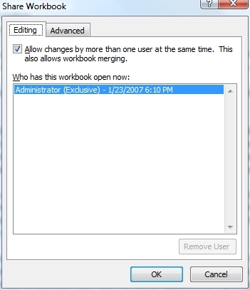
Figure A

To share the workbook, select the Allow Changes by More Than One User at a Time check box.

Before you click the OK key, go to the Advanced tab, shown in Figure B. As you can see in the figure, the Advanced tab asks you if you want to track changes to the file. If security is a concern to you, then I highly recommend tracking changes to the file. By doing so, you create an audit trail that allows you to see exactly what modifications were made by whom.
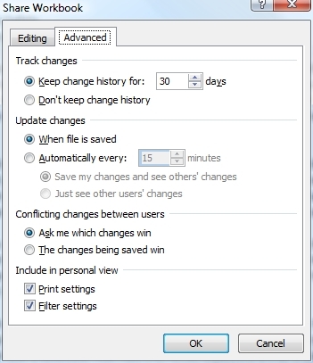

Figure B
The Advanced tab contains settings related to tracking document changes.

The next section is the Update Changes section. By default, updates occur when the file is saved, but you can configure changes to be updated on a periodic basis.

The fact that multiple users can work on the document simultaneously means that there is a potential for conflicts to occur. Two users could potentially save contradictory changes at the same time. As such, Excel makes you decide what should happen when contradictory changes occur. By default, Excel will ask you which change should be kept, but you have the option of configuring Excel so that the most recently saved change is authoritative. From a security perspective, I recommend going with the default setting because then you can decide for yourself which change to keep and which to discard.

The last section shown in Figure B is the Include in Personal View section. By default, each user is allowed to maintain his own separate printer settings and filtered view settings. This isn't usually a threat to security since a user cannot change another user's print settings or filter settings. Therefore, I recommend going with the default settings in this section.

Click OK, and the worksheet will be shared. Keep in mind, though, that you have only granted document-level sharing. It is still up to you to place the shared worksheet into a network location where it will be accessible to all of the necessary users. I strongly recommend setting some NTFS permissions so that only the intended users are allowed to access the document.

Enter text without changing the underlying cells in Excel 2007

Written by IT News on 9:34 PM

Excel cells are limited to 256 characters. However, the cell's size and ability to display its contents change with the size of its surrounding columns. Excel 2007's text boxes overcome these potential limitations.

For example, say you have allotted each department $5,000 per month for new computer equipment. The departments will need to start replacing notebook computers for the next release, and they will need to know how many they can replace on that budget. You decide to create a spreadsheet that calculates how much they can finance at the different interest rates they can obtain from local banks. Your spreadsheet lets each department enter a monthly payment within their equipment budget, and then click a button to get the result. To put these instructions into a text box at the top of the worksheet, follow these steps:

  1. Click the Insert tab and then click Text Box.
  2. Click and drag to draw a text box from D3:K6.
  3. Right-click the text box border.
  4. Click on Size And Properties.
  5. Under the Properties tab, click to select Move but don't size with the Cells button.
  6. Click Close.
  7. Right-click the text box border.
  8. Click Format Shape.
  9. Click Text Box.
  10. Click the Resize Shape To Fit Text check box and then click Close.
  11. Click within the text box to type your text. If the text extends below row 6, the box will expand vertically to accommodate the extra text. (Note: You can change the widths of the underlying columns, and the text box will retain its original size.)

Print what you see in Excel 2007's Page Layout View

Written by IT News on 3:24 AM

Excel 2007's Page Layout View allows you to avoid the frustration of creating unnecessary printouts of your spreadsheets. Here's an easy way to see your work (including headers and footers) using this view.

In versions of Excel prior to 2007, it is difficult to know how many printed pages it would take to print a spreadsheet unless you switch to Print Preview. It is only when you use Print Preview that you discover that the last column of your worksheet will print on page two. Also, you cannot create or even see your worksheet's headers and footers in Normal View.

Excel 2007 adds a new view called Page Layout, which allows you to see how your worksheet will print and lets you add a header and/or footer.

To see your spreadsheet as it would look on the printed page, follow these steps:

  1. Click the View tab.
  2. Click the Page Layout button in the Workbook Views section.

In Page Layout View, you can move the zoom slider to the left to display all of your worksheet pages. To add a header, click where it says Click To Add Header, and then type your text or click one of the buttons in the Header & Footer section to add it to the header. Here are three examples:

  • Click the Current Date button to insert the date at the center tab in the center cell of the header.
  • Press [Tab] to enter elements in the right-aligned cells of the header.
  • Press [Shift][Tab] to enter elements in the left-aligned cell of the header.

To create the footer, scroll to the end of the page and click where it says Click To Add Footer.


Customize Firefox using about:config

Written by IT News on 9:26 PM

One of the best things about Firefox is its flexibility and extensibility. Here's how you can tweak settings inside of Firefox using about:config. This article is also available as a TechRepublic download.

Internet surfers everywhere seem to be taken with Mozilla's browser offering, Firefox (now in release 2.0.x). This is partly due to the browser's speed and extensibility; but Firefox also has the ability to completely customize its configuration. This article will cover the last of Firefox's hidden pages, about:config and some of the tweaks it allows the user to make.

Accessing the configuration

To access the guts of the Firefox browser, enter about:config into the Address bar and press [Enter]. This will bring up a long list of customizable preferences for the current installation of the browser. The default configuration is similar the one shown in Figure A.

Figure A

Some options available in the default configuration of Firefox.

Note : Please click here to continue reading this article

Use index sheets to quickly navigate in an Excel workbook

Written by IT News on 6:16 PM

Help users increase productivity by automatically signing up for TechRepublic's free Microsoft Office Suite newsletter, featuring Word, Excel, and Access tips, delivered each Wednesday.

When working with large workbooks in Microsoft Excel, you can spend a good deal of time navigating through dozens of sheet name tabs to find the one you need. One method for making this task easier is to build an index sheet that contains hyperlinks to every worksheet in your workbook.

To create the index, follow these steps:

  1. Insert a new worksheet at the beginning of your workbook and rename it Index.
  2. Right-click on the sheet tab and select View Code.
  3. Enter the following code in Listing A.
  4. Press [Alt][Q] and save the workbook.

The next time you open the workbook, the Index sheet will contain a list of hyperlinks to each worksheet in the workbook. Each worksheet also contains a hyperlink back to the Index sheet. In this example, the link back to the Index is contained in cell H1, but it can be in any cell that is blank for all worksheets.

10 key enhancements in Excel 2007

Written by IT News on 5:42 PM

Given the learning hurdle that comes with an entirely revamped (albeit improved) user interface, Excel 2007 must offer significant enhancements to encourage you to upgrade. Herewith, my top 10.


To read this please click here

Turn off gridlines in your Excel applications

Written by IT News on 6:29 PM

Your users may find it easier to work with your worksheet applications if they can't see the gridlines. For example, let's say you developed a worksheet that displays a new chart that compares monthly sales figures for the department each time a salesperson enters his/her monthly sales figures. Your worksheet includes instructions for using the spreadsheet, a bordered cell where they are to enter their data, and the changing chart.

To prevent the salespeople from working with the other cells in the worksheet, you can turn off the gridlines in Excel 2003 or Excel 2002, by following these steps:

  1. Go to Tools | Options.
  2. On the View tab in the Windows section, clear the Gridlines check box.
  3. Click OK.

To turn off the gridlines in Excel 2007, follow these steps:

  1. Click the View tab.
  2. Clear the Gridlines check box in the Show/Hide section of the ribbon.

Miss a tip?

Check out the Microsoft Excel archive, and catch up on our most recent Excel tips.

Help users increase productivity by automatically signing up for TechRepublic's free Microsoft Office Suite newsletter, featuring Word, Excel, and Access tips, delivered each Wednesday.

50 essential Excel tips

Written by IT News on 11:22 PM

his message is loaded with valuable information that can save you time and effort. Below, you’ll find a sample of what the Excel TechMail has to offer. Get valuable tips on macros, formulas, formatting workbooks, links to Excel resources, and much more, all delivered straight to your inbox every weekday.

Search This Blog

Ads and Sponsored by:


Want to subscribe?

Subscribe in a reader.